With out freezing rows or columns in your Excel spreadsheet, every part strikes while you scroll by way of the web page, as proven within the gif under.

This may be irritating when you can’t at all times see key information markers that specify what information is what, like column headers or row titles.

As with many issues on Excel, there are methods that enable you to make your spreadsheets simpler to learn, just like the freeze operate. On this put up, learn to freeze rows and columns in Excel to make sure that, while you scroll round, you’ll at all times be capable of view the important thing information factors that matter most.

The best way to Freeze a High Row in Excel

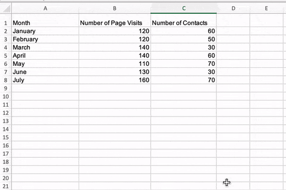
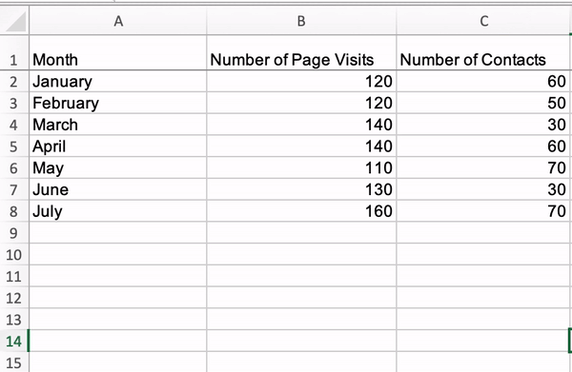
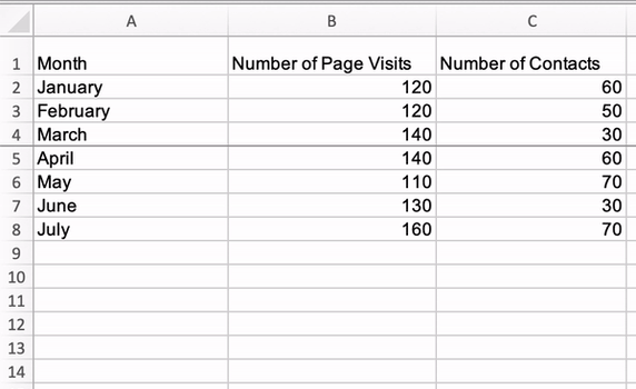
The picture under is the pattern information set I’ll use to run by way of the reasons on this piece.

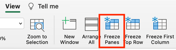
1. To freeze the highest row in an Excel spreadsheet, navigate to the header toolbar and choose View, as proven within the picture under.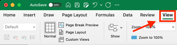

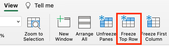
2. When the View menu choices seem, Click on Freeze High Row, outlined in crimson within the picture under.  

As soon as chosen, every part within the high row of your Excel spreadsheet (row 1) shall be frozen, and you’ll scroll up and down in your spreadsheet, however the high rows received’t transfer, as proven within the gif under.

The best way to Freeze a Particular Row in Excel

Whereas excel has native features for freezing the highest row of a knowledge set and the primary column of a knowledge set, there are further steps to take to freeze different components of your information set that aren’t these two issues.

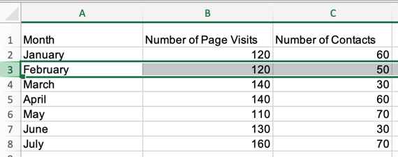
1. To freeze a particular row in Excel, choose the row quantity instantly beneath the one you need frozen. For this instance, I’m choosing row quantity three to freeze row quantity two.

2. After choosing your row, navigate to View within the header toolbar and choose Freeze Panes.

As soon as chosen, you’ll be capable of scroll up and down by way of your spreadsheet and at all times see row two.

Observe that utilizing the Freeze Panes operate to freeze rows additionally freezes each row above the row you initially chosen. For instance, within the gif under, I chosen row 5 which additionally freeze rows 4, three, two, and one.

The best way to Freeze the First Column in Excel

1. To freeze the primary column of your Excel spreadsheet (column A), navigate to the Excel header toolbar, choose View, and click on Freeze First Column.

As soon as chosen, you’ll be capable of scroll aspect to aspect inside your sheet, and the primary column of your information set will at all times be seen, as proven within the picture under.

The best way to Freeze a Particular Column in Excel

1. If you wish to freeze a particular column in excel, choose the column letter that’s instantly subsequent to the column you need frozen and click on Freeze Panes within the View header menu.

As soon as chosen, you possibly can scroll aspect to aspect by way of your complete information set and proceed to see these columns. Within the gif under, I’ve frozen columns A and B.

Utilizing the freeze operate in Excel makes your spreadsheets simpler to know, as you possibly can be certain that essential rows and columns are at all times seen as you scroll by way of your information.